Ray Tracing the Final Week

This is my third instalment of the ray tracing series. There are not many new tricks that I could share here as the final series is heavy on math, from Monte Carlo integration to importance sampling. I will try to explain the concepts as best as I can.

Scenes from Week 3

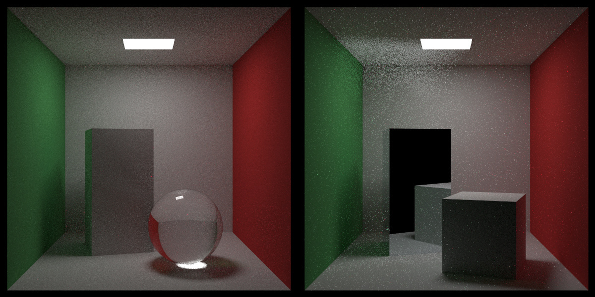
Problem statement

For scenes that are dark and with a few bright light sources, the image generated by the ray tracer is usually noisy. This is because the rays are randomly scattered and the number of rays that hit the light source is small and when the hit is missed, the returning value of that ray is going to be the background colour, which is usually black. When we construct the scene, we know exactly where the light sources are and we can use this information to our advantage. The idea is to send more rays to the light sources and mix up with the rays that are randomly scattered. This is called importance sampling.

Monte Carlo integration

The book starts with a classic example of Monte Carlo integration – estimating $\pi$. We know that the area of a unit circle is $\pi$ and the area of the enclosing square is 4. If we randomly throw darts at the square, the ratio of the number of darts that hit the circle to the total number of darts is going to be the ratio of the area of the circle to the area of the square. This is the idea behind Monte Carlo integration. We can use this idea to estimate the value of $\pi$ and we apply the same technique to estimate the value of the integral of an arbitrary function. To do that, we would need to draw samples from an arbitrary distribution. This is where sampling techniques come in. The following sections covers some of the sampling techniques that I learnt from this book and other sources.

Rejection sampling

Reject sampling, also known as rejection sampling, is a basic technique used in probabilistic sampling. It’s a method to generate observations from a distribution that might be difficult to sample from directly. The idea is to sample from a simpler distribution and then reject some of these samples based on a certain criterion. This method is particularly useful when the target distribution is complex, but you have a simpler distribution (called the proposal distribution) that is easy to sample from.

Here is a simple example written in Python:

import numpy as np
import matplotlib.pyplot as plt

def target_distribution(x):
    """ Probability density function of the target distribution: standard normal distribution """
    return np.exp(-x**2 / 2) / np.sqrt(2 * np.pi)

def proposal_distribution(x):
    """ Probability density function of the proposal distribution: uniform distribution between -3 and 3 """
    return 1/6 if -3 <= x <= 3 else 0

def reject_sampling(num_samples):
    samples = []
    while len(samples) < num_samples:
        x_proposal = np.random.uniform(-3, 3)  # Sample from the proposal distribution
        u = np.random.uniform(0, 1)  # Uniform random value for acceptance criterion

        if u < target_distribution(x_proposal) / (6 * proposal_distribution(x_proposal)):
            samples.append(x_proposal)

    return samples

# Generate samples
num_samples = 1000
samples = reject_sampling(num_samples)

# Plot the results
plt.hist(samples, bins=30, density=True, alpha=0.5, label='Sampled Data')
x = np.linspace(-3, 3, 1000)
plt.plot(x, [target_distribution(xi) for xi in x], label='Target Distribution')
plt.legend()
plt.show()

The result is shown below:

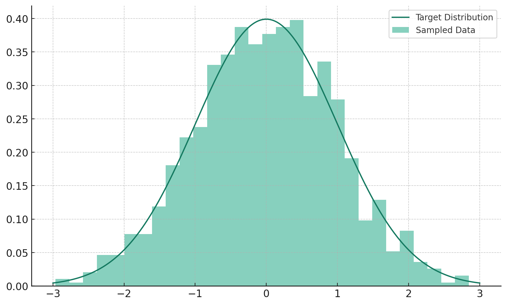rejection sampling

Inverse transform sampling

Invert sampling, often referred to as inverse transform sampling, is a method used in statistics and computational methods to generate samples from any probability distribution, provided that its cumulative distribution function (CDF) can be inverted. This method is particularly useful when you want to generate random samples from a complex distribution for which direct sampling is difficult.

Here is a simple example written in Python:

import numpy as np
import matplotlib.pyplot as plt

# Parameters
lambda_param = 1
num_samples = 1000

# Inverse CDF function for exponential distribution
def inverse_cdf(y, lambda_param):
    return -np.log(1 - y) / lambda_param

# Generate uniform samples
uniform_samples = np.random.uniform(0, 1, num_samples)

# Apply inverse CDF
samples = inverse_cdf(uniform_samples, lambda_param)

# Plot the histogram
plt.hist(samples, bins=30, density=True)
plt.title('Histogram of Samples from Exponential Distribution')
plt.xlabel('Value')
plt.ylabel('Density')
plt.show()

The result is shown below:

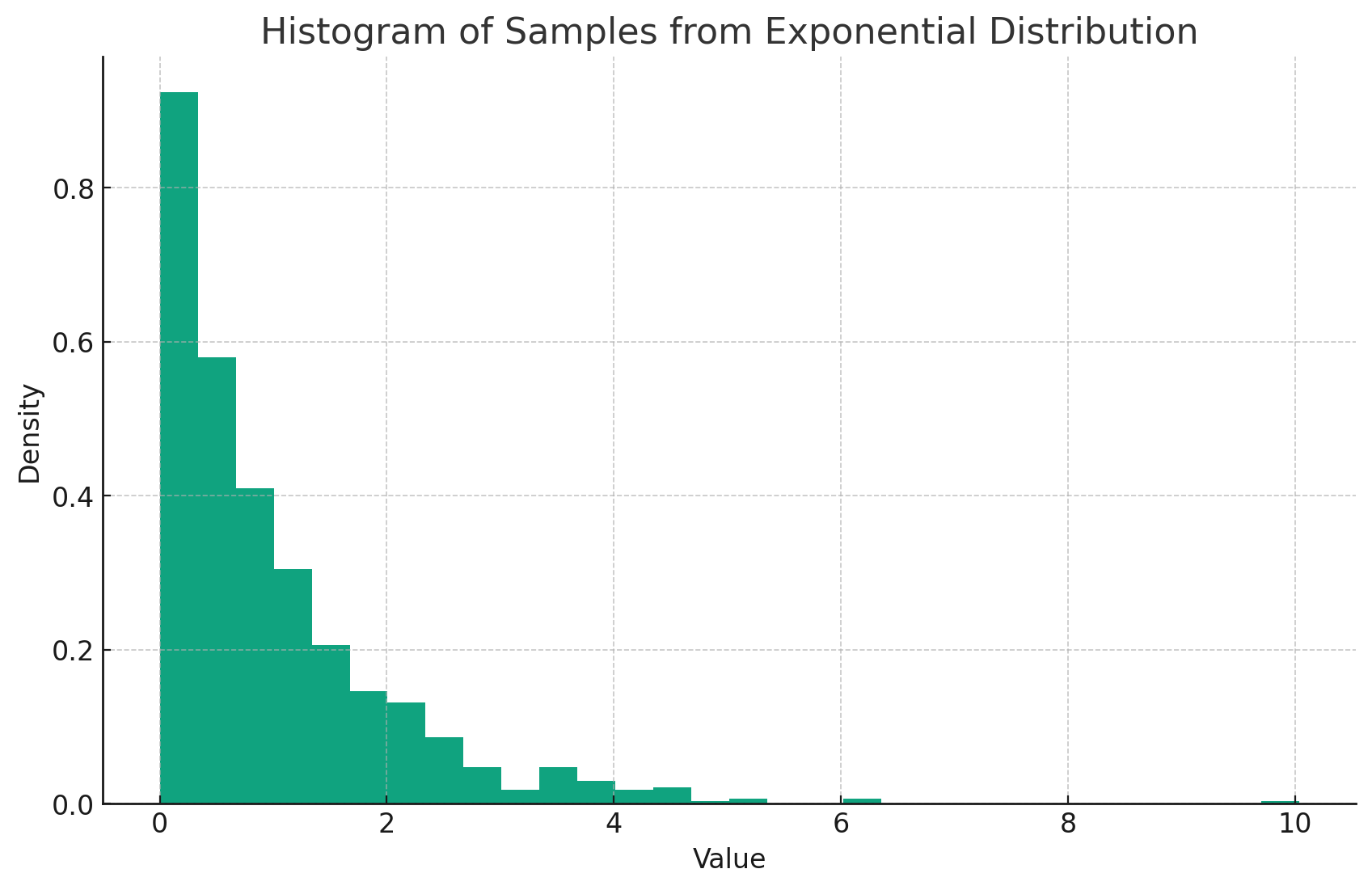inverse transform sampling

Metropolis-Hastings algorithm

The Metropolis-Hastings algorithm is a Monte Carlo method used for obtaining a sequence of random samples from a probability distribution for which direct sampling is difficult. This sequence can be used to approximate the distribution (e.g., to calculate integrals).

Here is a simple example written in Python:

import numpy as np
import matplotlib.pyplot as plt

def target_distribution(x):
    """ Target distribution: Gaussian with mean 0 and std deviation 1 """
    return np.exp(-0.5 * x**2) / np.sqrt(2 * np.pi)

def metropolis_hastings(target_pdf, initial_guess, iterations, proposal_width):
    """ Metropolis-Hastings Algorithm """
    current_state = initial_guess
    samples = []

    for i in range(iterations):
        # Propose a new state
        step = np.random.normal(loc=0, scale=proposal_width)
        candidate_state = current_state + step

        # Calculate acceptance probability
        accept_probability = min(target_pdf(candidate_state) / target_pdf(current_state), 1)

        # Accept or reject the new state
        if np.random.rand() < accept_probability:
            current_state = candidate_state

        samples.append(current_state)

    return samples

# Parameters
initial_guess = 0
iterations = 10000
proposal_width = 1

# Run the Metropolis-Hastings algorithm
samples = metropolis_hastings(target_distribution, initial_guess, iterations, proposal_width)

# Plotting
plt.hist(samples, bins=30, density=True)
plt.title("Metropolis-Hastings Sampling")
plt.xlabel("Value")
plt.ylabel("Density")
plt.show()

The result is shown below:

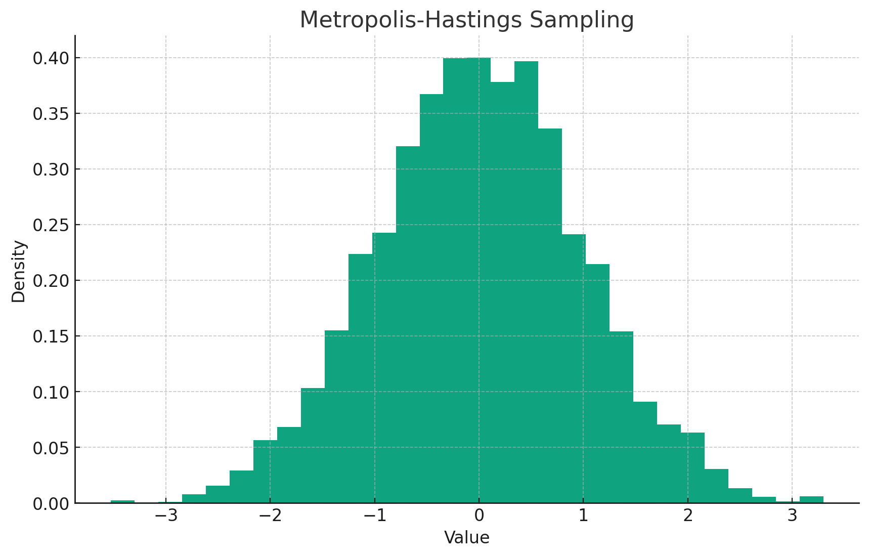metropolis-hastings sampling

Implementation

The implementation itself isn’t too interesting. One thing worth pointing out is that dielectrics and metals are specular materials and they are not diffuse and to make it work, the code introduces something called skip_pdf to skip the sampling process. And for lamberian materials, the code uses cosine weighted sampling to sample the direction of the scattered ray from spheres and mix up with light sources.

In Peter Shirley’s code, he uses a virtual pointer for the PDF in a scattering record. It works for normal C++ but with CUDA, having to new in device context is 10x slower. Hence, to solve this problem, I adapted manual polymorphism using switch :). Another challenge is to unwind the recursive code into linear code. As more branching is added in the later chapters, it became a bit tricky to unwind the code. I think I have done a decent job in this regard.

Final thoughts

It has been a fantastic journey reading and implementing Peter Shirley’s ray tracing books. There are certainly more things to dig up and learn just like what Peter said in his last book. For me, I think there are a few things that I would like to explore further:

remove the use of virtual functions and use simple dispatching instead
build BVH tree directly in device and avoid transfering back and forth between host and device
explore nested BVH tree and see if it can improve performance
implement triangle mesh
learn optix

I hope you have enjoyed reading this series as much as I have enjoyed writing it. I will be taking a break from ray tracing and will be focusing on other topics. Until then, happy ray tracing!