Ray Tracing wih CUDA 101
Ray Tracing with CUDA (101)
My journey into the realm of parallel programming has been a thrilling one, fueled by years of fascination and a drive to harness the power of multi-core CPUs in my everyday work. This passion took root during my PhD research, where I delved into High Performance Computing (HPC) and experimented with MPI, stretching calculations across multi-node clusters. As a professional software developer and an avid PyTorch user, I’ve come to appreciate how PyTorch leverages GPU capabilities and efficiently utilizes all available computer cores. However, this convenience comes with a level of abstraction that leaves me yearning for a deeper understanding of the underlying mechanisms.
Seeking to quench this thirst for knowledge, I embarked on a learning adventure with Caltech’s CUDA course, which proved to be an eye-opener. This experience inspired me to explore further applications of this technology, leading me to the fascinating world of ray tracing - a concept I’ve been enamored with since my days playing video games. GPUs, with their innate knack for graphics rendering and parallel computing, are perfectly suited for this task.
In my quest for comprehensive understanding, I stumbled upon the legendary “one weekend” series of posts by Peter Shirley. To date, I have devoured the first two series, applying my newfound CUDA skills to implement the code for the initial series and the BVH tree for the sequel. Roger Allen’s CUDA implementation served as my springboard into this exciting domain, and I highly recommend his enlightening post on the NVIDIA tech blog here.
Now, I am poised to chronicle my experiences and insights in a series of posts, hoping to enlighten and inspire those who share an interest in this captivating topic.
CPU -> GPU
Understanding the distinction between CPUs and GPUs in computing is like comparing a skilled multitasker to a team of specialized workers. CPUs, akin to a versatile multitasker, excel at handling a few complex tasks simultaneously. They boast a limited number of cores, often ranging from 4 to 12 in typical desktop computers. Each core is a powerhouse in its own right, capable of performing multiple operations simultaneously, a feat known as hyper-threading. CPUs shine in sequential tasks, thanks to their rich instruction sets and sophisticated branch prediction algorithms.
Conversely, GPUs resemble a large team of workers, each focused on a simple, specific task. With potentially thousands of cores, GPUs can handle numerous tasks at once, albeit each core is limited to one task at a time. For instance, the Intel i7-8700K CPU has 6 cores, each operating at 3.7 GHz. In contrast, the GeForce GTX 1080 Ti, a GPU from yesteryears, boasts 3584 cores, although at a lower 1.48 GHz each.
When it comes to executing a single task, CPUs often outpace GPUs. However, GPUs take the lead in scenarios requiring the simultaneous execution of many tasks, particularly in fields like matrix operations and graphics rendering. It’s important to note that GPUs aren’t universally faster than CPUs; their efficiency depends on the nature of the task and its implementation. Tasks that are predictable and computationally intensive are prime candidates for GPU acceleration.
Ray Tracing
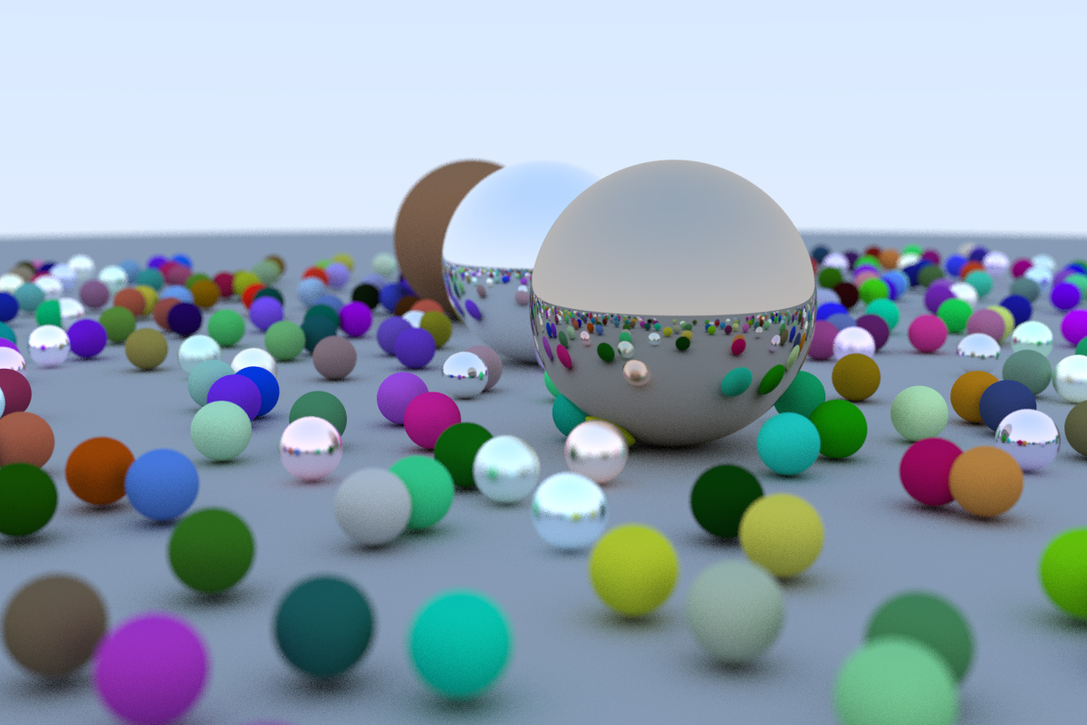
Ray tracing, a marvel of computer graphics, operates on a fascinating principle: each ray emanating from the camera navigates the scene independently, potentially numbering in the hundreds of thousands for a typical setup. The core concept is simple yet profound - tracing light’s journey and simulating its interactions with objects. Imagine a ray projected from the camera, exploring the scene for object encounters. Upon impact, it assesses the object’s color at the point of contact, then launches a new ray from there to further probe the environment. This iterative process continues until the ray either illuminates from a light source or exhausts its maximum bounce limit. The pixel’s hue then reflects either the light source’s color or, in the absence of a hit, the background’s. For a deeper dive into this technique, as well as its counterpart ‘rasterization’, the Wikipedia pages on rasterization and ray tracing offer comprehensive insights.
The interaction between rays and objects can initially follow a ‘brute force’ approach - a thorough but sluggish method of scanning every object, as showcased in Peter Shirley’s first series. The alternative, a Bounding Volume Hierarchy (BVH) tree, introduces efficiency, introduced in the second embarkment. By segmenting the scene into smaller boxes, this method rapidly assesses potential ray interactions, examining objects within a hit box and bypassing empty ones. This approach resembles a binary search algorithm tailored for ray tracing, and is detailed in Shirley’s second series. Dive into the specifics of BVH trees here.
Implementing BVH trees on GPUs, however, poses challenges due to their recursive and memory-intensive nature. To enhance efficiency in my CUDA adaptations, I transformed the tree structure into a linear array. This ‘linearization’ process involves constructing the tree on the CPU, then flattening it for GPU usage, yielding significant performance improvements. To illustrate the impact of these optimizations on my setup (AMD5800X, RTX3080, 32GB RAM), here’s a comparison using a test scene (1200x800 pixels, 488 random spheres, 100 samples per pixel, 50 max bounce limit):
- Pure CPU (brute force): ~4min40s (single core; extrapolated from 10 to 100 samples per pixel)
- Unoptimized CUDA: ~15s (GPU)
- Optimized CUDA (brute force): ~6s (GPU)
- Optimized CUDA with BVH tree: ~0.5s (GPU)
Clearly, GPUs outperform CPUs, and the BVH tree method significantly trumps the brute force approach in speed.
CUDA Insights
My exploration with CUDA has yielded some valuable insights I’d like to share:
- Memory Access and Optimization: The choice of grid, block, and thread sizes in CUDA is crucial, as memory access patterns significantly impact performance. However, it’s important to find a balance and avoid excessive optimization.
- Memory Allocation: Opt for
cudaMallocinstead of dynamic memory allocation. In my experience,cudaMallocis noticeably faster. - Parallelization Strategy: Parallelizing over rays, rather than over pixels or samples, has proven more effective. This approach aligns better with CUDA’s architecture.
- Code Compilation: Compiling each
.cufile into a.ofile and then linking them yields faster code. While Roger Allen prefers header files for simplicity and clarity, I’ve found that separating.hand.cufiles and using aMakefilefor compilation and linking enhances performance.
Final Thoughts
This journey through CUDA and ray tracing has been incredibly enriching. I’ve not only learned a great deal but also enjoyed every step. Once I complete the implementation of the final scene from Peter Shirley’s second book, I plan to release all my code to the public. In the meantime, I welcome any questions or suggestions. Engaging in discussions and sharing knowledge with fellow enthusiasts is something I always look forward to.